CS7641 - Project Team 17
Introduction
At present, the visually impaired people use a simple stick for navigation. However, the use of such a stick does not enable them to navigate independently. If they ever get into an unknown environment, the most that they can do, without any external help, is detect stationary obstacles around them. Unfortunately, they cannot make any decision based on a comprehensive understanding of the environment.
To address this problem, we intend to develop a Machine Learning model for generating accurate visual understanding of a given scene. A model of this kind can potentially be integrated into an e-stick which assists the visually impaired and enables them to move with the same ease and confidence as normally sighted people.
Problem Definition
Our project aims at developing a software framework that can detect objects from images and then answer questions based on the content of those images. From a big picture perspective, this project is a stepping stone towards engineering a system that can capture real-time images to provide high-level contextual information about the surroundings. In the future, combining such a system with a mapping and navigation module and integrating into an e-stick would enable the visually impaired to navigate independently.
Dataset
To resolve the visual challenges faced by the visually impaired people in their day-to-day lives, we present a Machine Learning model based on the Vizwiz dataset. The training dataset consists of photos taken by the blind people annotated with the question asked relevant to that image. Each annotation question also consists of answers and answer types specified by 10 people for each sample. This provides an opportunity as well a challenge to assist the visually impaired to help them in navigation, assisting their daily life tasks and answering their visual questions etc. The original Vizwiz dataset consisted of :
Methods
Step 1. Data Preprocessing
Feature Extraction using Convolutional Neural Networks
We use transfer learning to create feature vectors for the images present in the dataset. The activations from the last layer of different 3 pre-trained models like Inceptionv3, ResNet (Residual Network) and VGG16 (Very Deep Convolutional Networks for Large-Scale Image Recognition), which are state-of-the-art and are widely used. These models are pre-trained on ImageNet, which is a huge image dataset containing more than 14 million images. Hence, they can be used for our task to create feature vectors of the images considered for our task from the Vizwiz dataset.
We first ran the Inceptionv3 using CPU and GPU, with and without batching. The time taken for each of these operations are displayed in Table 1. We also tried out different batching sizes while running the feature extraction, this information is displayed in Table 2.
| CPU/GPU used | Time |
|---|---|
| CPU feature extraction time | 1 h 42 min |
| CPU feature extraction time | 43 min |
| Batching Sizes | Time |
|---|---|
| 4 | 8m 2s |
| 8 | 5m 9s |
| 16 | 5m 14s |
| 32 | 5m 11s |
| 64 | 5m 2s |
Unsupervised Algorithm: Clustering
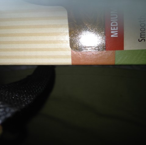
On closely examining the dataset, we observed that few images are totally blurred, few are black/white and few others just have too much flash. Hence we realised the need to clean the dataset before feeding it to our training pipeline.
Challenge 1:
The first challenge that we faced is how to identify the images to be discarded.
Solution:
Challenge 2:
K-means clustering uses Euclidean distance as the metric to determine the similarity between different images. But some images might contain similar objects but they might be present in different orientations/positions/color contrasts, etc. Hence considering just the euclidean distance between the pixel values is not a good metric.
Solution:
We used CNN to detect and classify the objects and accordingly performed the clustering on these CNN generated feature vectors. Each CNN layer performs optimized operations like centering the objects, gray-scale conversion(normalization), detecting the objects, and accordingly classifying and clustering the images.
Challenge 3:
The next challenge that we faced was to identify the correct value of K(number of clusters) to be generated.
Solution:
To identify the accurate number of clusters to be considered, we calculated the loss values for a variety of distinct K values. We then plotted each of these values and used the Elbow method to determine the best value of K to be considered for our use case.
The following table depicts the loss values obtained for each value of k:
| Value of K (Number of Clusters) | Loss Value |
|---|---|
| 1 | 7674 |
| 2 | 7501 |
| 3 | 7411 |
| 5 | 7268 |
| 10 | 7051 |
| 20 | 6830 |
| 40 | 6612 |
| 60 | 6477 |
| 300 | 5957 |
| 1000 | 5494 |
The following is the elbow curve we generated based on the above values:
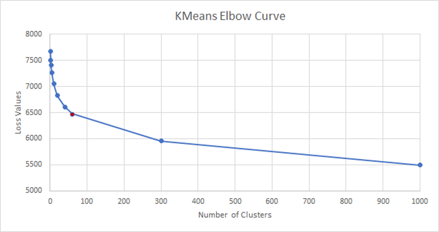
Hence, based on the elbow method, we obtained the accurate value of K as 60. Therefore, we generated 60 clusters. We then manually visited each of the clusters(i.e. each of the 60 folders of images), and discarded a few clusters to create a clean image dataset. In this way, the dataset was reduced from 20,523 image/question pairs to 13000 image/question pairs.
The following images show samples that were discarded:

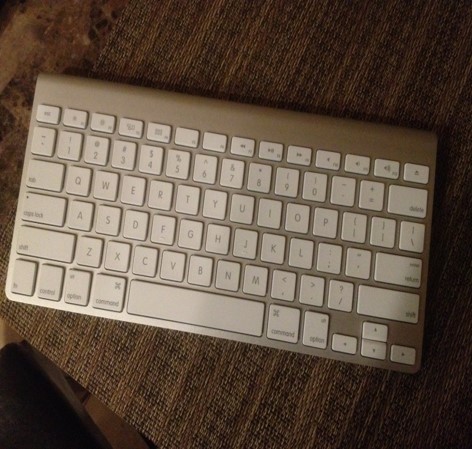
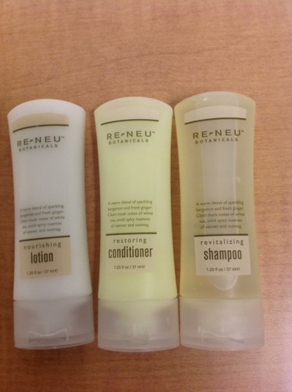
The following images show samples that were included:
Results of Data preprocessing
To overcome challenges 1,2 and 3 we ran K-means on feature vectors generated by a forward pass of a Convolutional Neural Network to generate 60 clusters, and out of those 60 clusters, we kept 29 clusters and discarded the rest based on the reasoning provided before, thus generating a dataset consisting of 13000 image/question pairs.
Annotation Script
After generating 29 folders(clusters), we had to use only the images from these folders. To uniquely read images from 29 out of 60 folders, we wrote an annotation script.
The script reads the annotation json file, which consists of the following structure:
{
Image_name : “ “, // Image name
“Question: “ “, // The question associated with each image
“Answers” : {
		// List of answers from 10 people
	      }
“Answer_type”:[ yes/no], [other], [unanswerable],
“Answerable” : 0/1
}
From this file, only those images will be considered that are present in the 29 clusters, and for those image names, we read questions and answers associated with them. All this data is then loaded into a new json file.
This new json file is then used for further processing.
Verification of Clustering using PCA and T-SNE
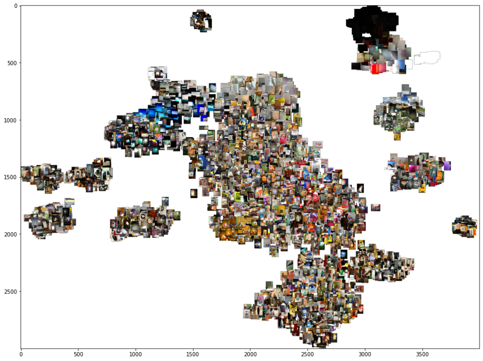
Post k-means clustering, we selected a few clusters manually. In order to verify that the clusters selected manually were accurate, we used PCA to reduce the dimensionality and then t-SNE to visualize the high-dimensional data of images into clusters.Principle Component Analysis(PCA)
PCA is the process of dimensionality reduction in which we can project each data point onto only to the first few principal components to obtain lower-dimensional data while preserving maximum datas variation. Here, we use PCA to reduce the dimensionality of the feature vectors of the images, so that the feature vectors can then be given as input to T-SNE.
T-SNE:
T-SNE is an unsupervised, non-linear technique primarily used for data exploration and visualizing high-dimensional data. The t-SNE algorithm calculates a similarity measure between pairs of instances in the high dimensional space and in the low dimensional space. It then tries to optimize these two similarity measures using a cost function. t-SNE differs from PCA by preserving only small pairwise distances or local similarities whereas PCA is concerned with preserving large pairwise distances to maximize variance.
In the figure below we can see that the clusters selected manually are well-defined, and hence we can clearly state that the clustering has been done accurately. We also tried tuning the hyperparameters by giving different values for (no. of clusters), to obtain different results.
Average and Max Pooling
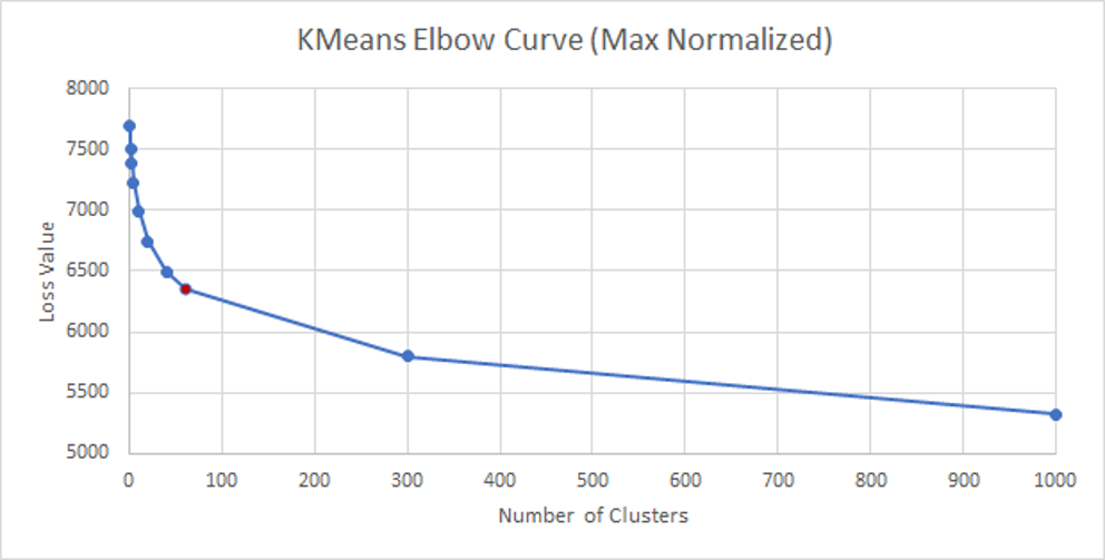
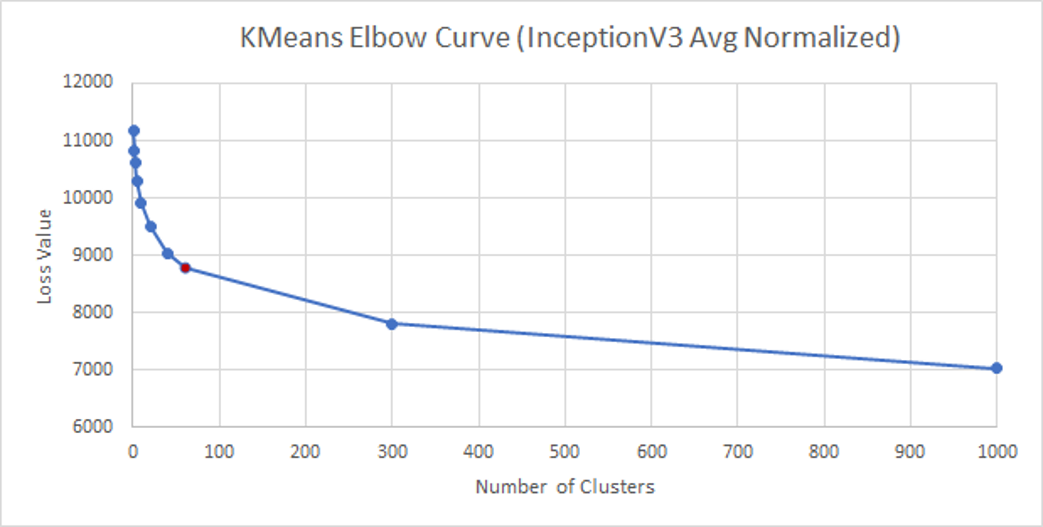
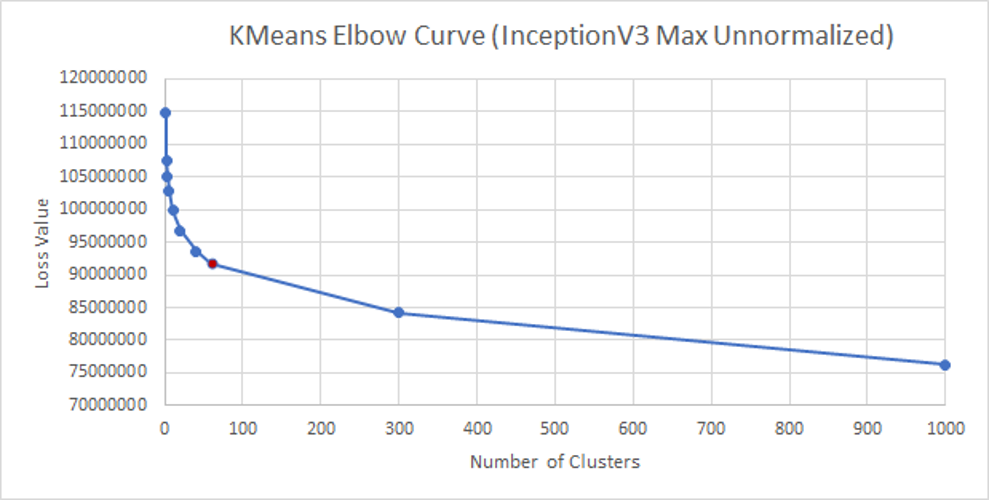
We also experimented taking max pooling and average pooling post the convolution layers for both Inceptionv3 and ResNet models, the results of which are shared in Tables 4, 5, 6, 7 and 8.
Resnet V/s Inception
InceptionV3_Max_Normalized
| Value of K (Number of Clusters) | Loss Value |
|---|---|
| 1 | 7691 |
| 2 | 7508 |
| 3 | 7392 |
| 5 | 7226 |
| 10 | 6991 |
| 20 | 6747 |
| 40 | 6499 |
| 60 | 6356 |
| 300 | 5796 |
| 1000 | 5322 |
InceptionV3_Avg_Normalized
| Value of K (Number of Clusters) | Loss Value |
|---|---|
| 1 | 11171 |
| 2 | 10832 |
| 3 | 10630 |
| 5 | 10307 |
| 10 | 9913 |
| 20 | 9508 |
| 40 | 9046 |
| 60 | 8788 |
| 300 | 7813 |
| 1000 | 7029 |
InceptionV3_Max_Unnormalized
| Value of K (Number of Clusters) | Loss Value |
|---|---|
| 1 | 114840986 |
| 2 | 10739880 |
| 3 | 105134892 |
| 5 | 102756470 |
| 10 | 99803204 |
| 20 | 96764906 |
| 40 | 93636811 |
| 60 | 91779277 |
| 300 | 84182650 |
| 1000 | 76288868 |
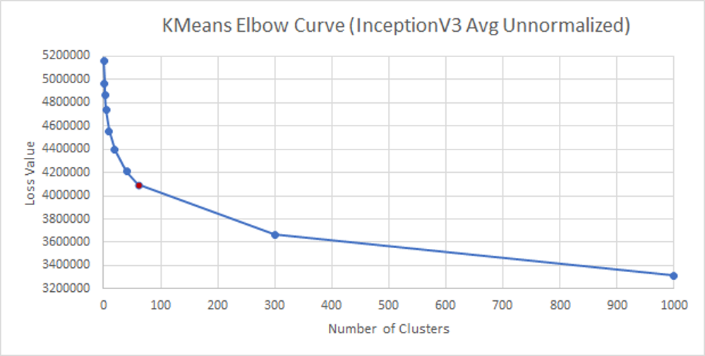
InceptionV3_Avg_Unnormalized
| Value of K (Number of Clusters) | Loss Value |
|---|---|
| 1 | 5165279 |
| 2 | 4968424 |
| 3 | 4867648 |
| 5 | 4738606 |
| 10 | 4554972 |
| 20 | 4392889 |
| 40 | 4207680 |
| 60 | 4094941 |
| 300 | 3667674 |
| 1000 | 3312151 |
ResNet50_Max_Normalized
| Value of K (Number of Clusters) | Loss Value |
|---|---|
| 1 | 2840 |
| 2 | 2218 |
| 3 | 2026 |
| 5 | 1855 |
| 10 | 1679 |
| 20 | 1537 |
| 40 | 1421 |
| 60 | 1361 |
| 300 | 1146 |
| 1000 | 960 |
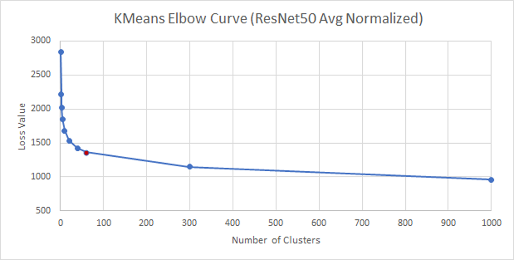
We finally use Inceptionv3 with max-pooling and run it on GPU using 32-sized batches. K-Means is run on these image feature vectors and based on the loss values received, we selected this architecture.
2. Training Pipeline:
After choosing the relevant clusters, the next task is to represent the training data to be fed into the neural network. We will be using the CNN features along with Question Text features as our input features. We will fuse these vectors together by simply stacking the matrices.
Question Representation
Bag of Words
To generate BOW for questions, we have used the following steps:
Limitations of Bag of Words
Using the bag-of-words technique has the following two limitations:BERT Question Embeddings
We use SentenceBERT to encode all questions into 768-dimensional word embeddings. SentenceBERT takes sentences as an input (it can take a sentence pair as well). These sentences are then passed into a BERT model and a pooling layer to generate embeddings. BERT stands for Bidirectional Encoder Representations from Transformers. It is a transformer-based machine learning technique for natural language processing pre-training developed by Google. SentenceBERT uses siamese and triplet network structures to derive semantically meaningful sentence embeddings that can be compared using cosine-similarity. Using sentence embeddings in BERT requires pre-processing such as adding tokens like [CLS] and [SEP] tokens, denoting the start and end of the sentence. We use the BERT tokenizer to tokenize the sentences. We take the last hidden layer of SentenceBERT to compute the embeddings. These embeddings are of dimension 768 for each question sentence.
Answer Representation
Similar to Question text representation, we also need to model answer text. The unique thing about the Vizwiz dataset is that for each question, we have 10 answers that are annotated. So we have multiple ground truth labels for each question. We decided not to use One hot encoding because that would lead to very high dimensional label vectors, blowing up the feature space and making the model suffer from the curse of dimensionality. Thus, we followed the following steps:
Architecture
As discussed in the training pipeline, we have the image + question embedding for each of the (image, question) pairs. For image embeddings, we use the frozen parameters from the Inceptionv3 model learned on ImageNet classification, and no fine-tuning was performed.
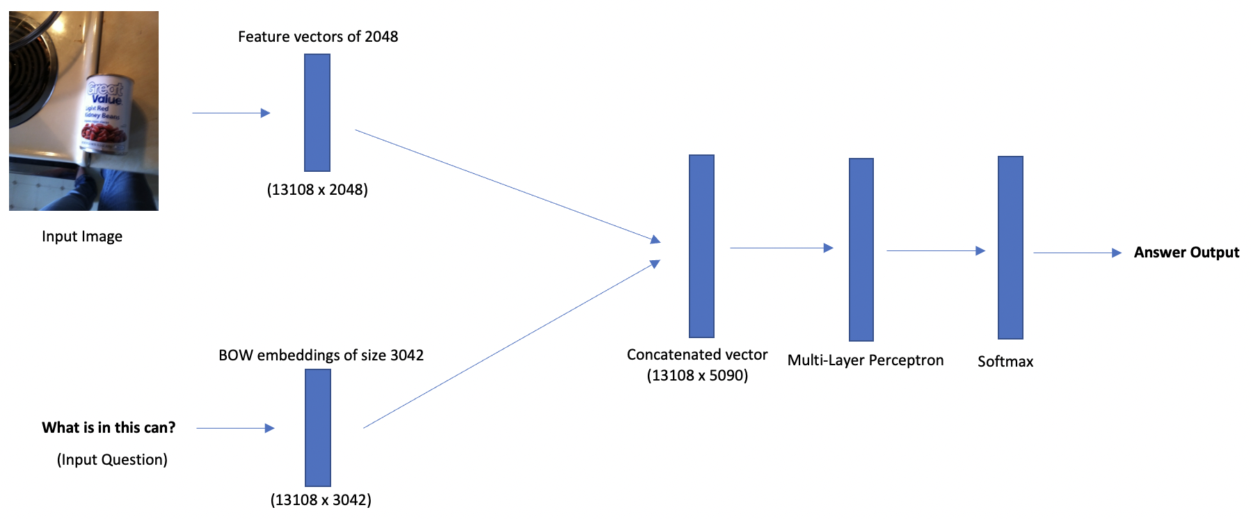
Previous Architecture using Bag-of-Words
We concatenate the BOW questions and images (2048 + 3042), to get a resultant vector of dimension 5090. We use this combined input for the Multi-Layer Perceptron (MLP). MLP is a fully connected neural network classifier consisting of 4 hidden layers with 5090 hidden units. We use ReLU for activation, which is finally followed by a log softmax layer to obtain a probability distribution over the top K answers. Since the VizWiz dataset has 10 ground-truth answers for each training instance, we use a "soft" cross-entropy loss so that the model optimises the weights by considering each ground-truth answer.
Current Architecture using BERT Embeddings
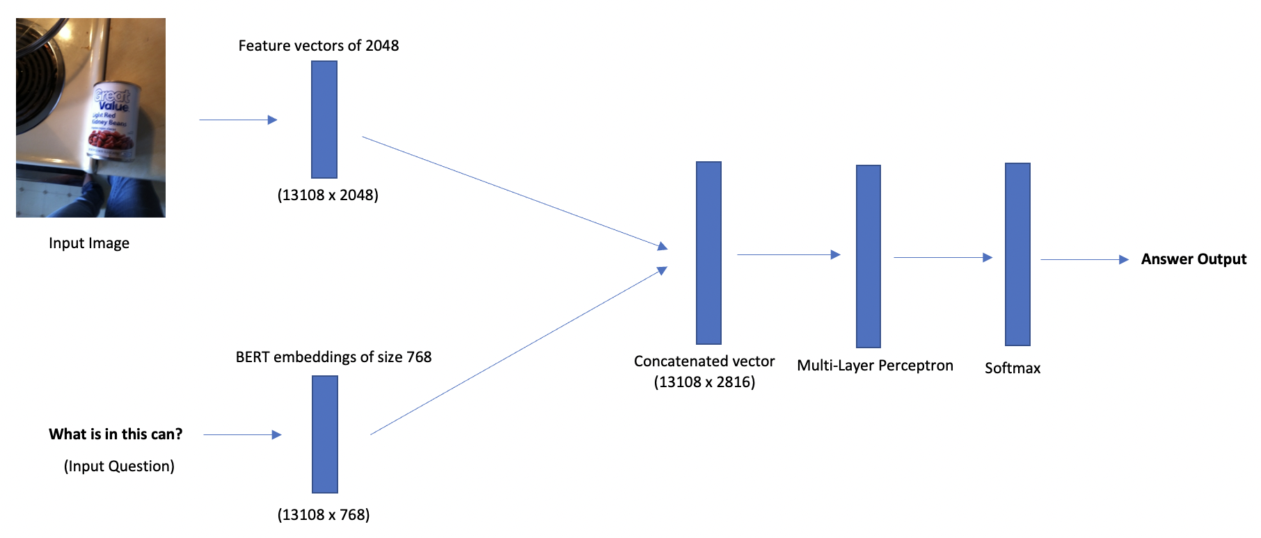
in the current architecture we integrate the BERT question embeddings and images (2048 + 768), to get a resultant vector of dimension 2816. Here, we have generated results by changing the number of hidden layers, hidden units, neurons, drop-out rates, learning rates as well as with/without regularization. Similar to the previous architecture, we use ReLU as the activation function, which is followed by a log softmax layer to obtain a probability distribution over the top K answers.
Loss Function Used
The proposed loss function, termed as soft cross entropy, is a simple weighted average of each unique ground-truth answer.

here c is a vector of unique ground-truth answers and w is a vector of answer weights computed as the number of times the unique answer appears in the ground-truth set divided by the total number of answers.
Accuracy Metric Used
The 10 answers given by humans for each visual question can differ and therefore, a prediction to a visual question can be 100% correct if the answer has at least 3 occurrences, ∼67% if the occurrences are exactly 2, ∼33% if the answer appears only once in the sample annotations. Hence, we use the following accuracy metric:

Preliminary Results for Mid-term
The following are the preliminary results of training on randomly selected samples from the filtered VizWiz dataset.
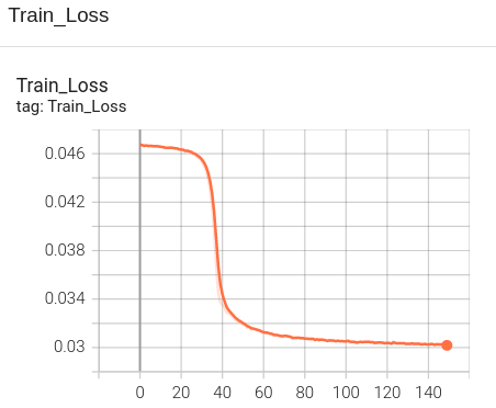
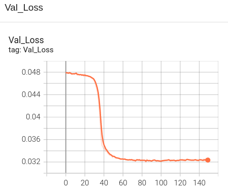
Final Results
BERT and BOW Models without dropout and regularization
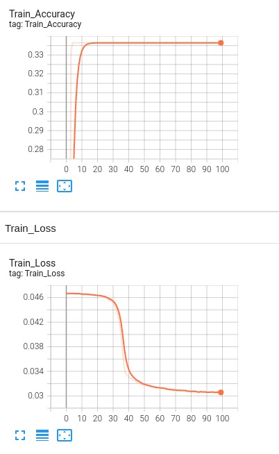
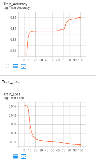
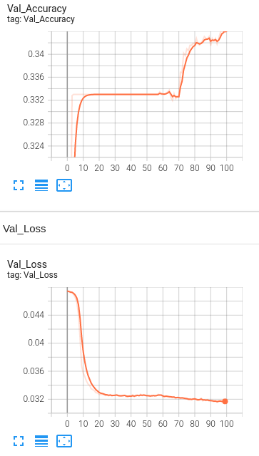
Model 1: Baseline Accuracy Graph for epochs = 100, 4 Hidden Layers for training dataset without dropout and regularization
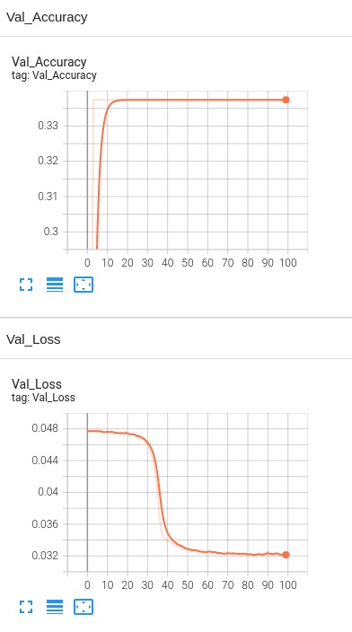
Baseline Accuracy Graph for epochs = 100, 4 Hidden Layers for validation dataset without dropout and regularization
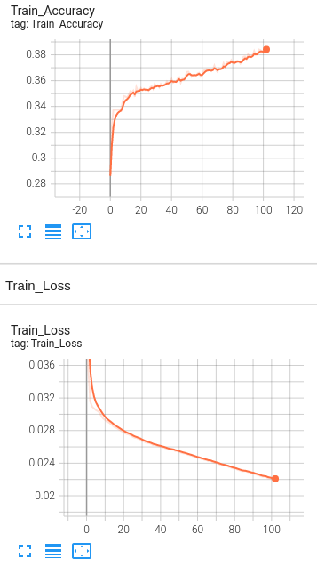
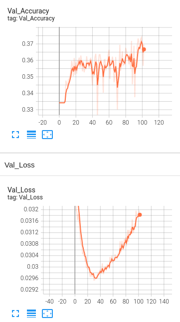
Model 2: BERT Accuracy Graph for epochs = 100, 4 Hidden Layers for training dataset without dropout and regularization
BERT Accuracy Graph for epochs = 100, 4 Hidden Layers for validation dataset without dropout and regularization
BERT and BOW Models with dropout and regularization
Model 1: 4 Hidden Layers with BOW with Learning rate set to 1e-6.

Model 2: 4 Hidden Layers with BERT embeddings with Learning rate set to 1e-5.
Model 3: 4 Hidden Layers with BERT embeddings with Learning rate set to 1e-4.
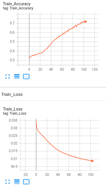

Model 4: 1 Hidden Layer with BERT embeddings , Learning rate set to 1e-5 and number of neurons set to 5000.
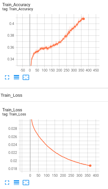
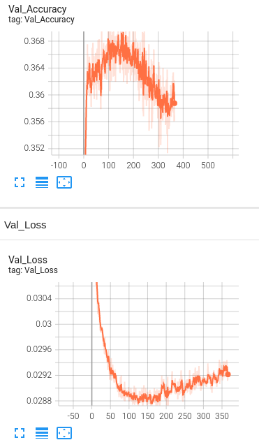
Model 5: 1 Hidden Layer with BERT embeddings, drop out layers(0.5) , Learning rate set to 1e-5 and number of neurons set to 3000 and L2 regularization(1e-5).
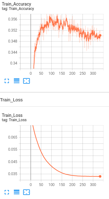
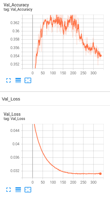
Model 6: 1 Hidden Layer with BERT embeddings, drop out layers(0.5) , Learning rate set to 1e-5 and number of neurons set to 1024 and L2 regularization(1e-5).

Model 7: 1 Hidden Layer with BERT embeddings, drop out layers(0.5) , Learning rate set to 1e-5 and number of neurons set to 1024 and L2 regularization(1e-5) only on training loss.

Model 8: 1 Hidden Layer with BERT embeddings, drop out layers(0.5) , Learning rate set to 1e-5 and number of neurons set to 512 and L2 regularization(1e-5).

Model 9: 1 Hidden Layer with BERT embeddings, drop out layers(0.5) , Learning rate set to 1e-5 and number of neurons set to 256 and L2 regularization(1e-5).

Model 10: 2 Hidden Layers with BERT embeddings, drop out layers(0.5) , Learning rate set to 1e-5 and number of neurons set to 128 and L2 regularization(1e-5).

Model 11: 1 Hidden Layers with BERT embeddings, drop out layers(0.5) , Learning rate set to 1e-5 and number of neurons set to 128 and L2 regularization(1e-5).

Accuracy Analysis:
The baseline accuracy is around 33%, and the final accuracy of the model with BERT is 35.8%. We see only a slight increase in the accuracy. Since the visually impaired people take pictures as well as ask questions themselves, the dataset being used is a challenging dataset for modern vision algorithms. It imposes the following challenges for model's training:
Conclusion and Future Scope
In this way our project aims at developing a software framework that can detect objects from images and then answer questions based on the content of those images. From a big picture perspective, this project provides high-level contextual information about the surroundings to the visually impaired.
Following are some ways we can work on the future aspects of the project: